cs285-lec8-DRL with Q-Functions

Summary

Q learning with:

• replay buffer
• target networks
• double networks
• continuous actions

Then we get ddpg:

1. take some action $a_i$ and observe $(s_i, a_i, s'_i, r_i)$, add it to $\mathcal{B}$, the actions were generated by $\phi$ and we might use epsilon-greedy here.
2. sample mini-batch $(s_j, a_j, s'_j, r_j)$ from $\mathcal{B}$ uniformly
3. compute $y_j = r_j + \gamma Q_{\phi'}(s'_{j}, \mu_{\theta'}(s'_j))$ using target network $Q_{\phi'}$ and $\mu_{\theta'}$
4. $\phi \leftarrow \phi - \alpha \sum_j\frac{\partial Q_\phi(s_j, a_j)}{\partial \phi}(Q_\phi(s_j, a_j) - y_j)$
5. $\theta \leftarrow \theta + \beta \sum_j \frac{\partial{Q_\phi}}{\partial{\theta}}$
6. update $\phi', \theta'$: eg Polyak averaging

Replay Buffer

In online q-learning we have:

1. take an action $a_i$ and observe $(s_i, a_i, s'_i, r_i)$
2. $y_i = r_i + \gamma \max_{a'}Q_\phi(s'_i, a'_i)$
3. $\phi \leftarrow \phi - \alpha \frac{\partial Q_\phi(s_i, a_i)}{\partial \phi}(Q_\phi(s_i, a_i) - y_i)$

to combine step2 and step3, we get:

1. take an action $a_i$ and observe $(s_i, a_i, s'_i, r_i)$
2. $\phi \leftarrow \phi - \alpha \frac{\partial Q_\phi(s_i, a_i)}{\partial \phi}(Q_\phi(s_i, a_i) - \underbrace{[r_i + \gamma \max_{a'}Q_\phi(s'_i, a'_i)])}_{\text{target value}}$

Because all the samples we collected are happened sequentially, they are similar and strongly correlated, and the target value is always changing.

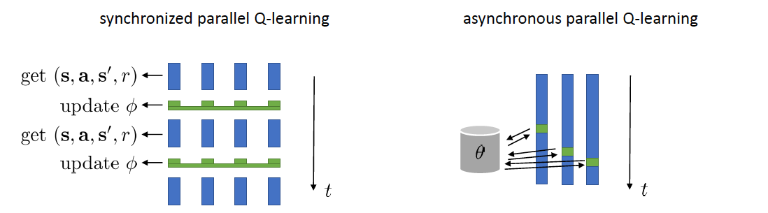
synchronized/asynchronized parallel Q-learning
To solve this problem, we could use synchronized parallel Q-learning or asynchronized parallel Q-learning as used in actor-critic:

replay buffer
Use replay buffers to generate data samples, we now have:

1. sample a batch $(s_i, a_i, s'_i, r_i)$ from $\mathcal{B}$
2. $\phi \leftarrow \phi - \alpha \sum_i\frac{\partial Q_\phi(s_i, a_i)}{\partial \phi}(Q_\phi(s_i, a_i) - [r_i + \gamma \max_{a'}Q_\phi(s'_i, a'_i)])$

This way samples are no longer correlated, and due to multiple samples in one batch, we have low-variance.

In the end, we get the full q-learning with replay buffer:

Large replay buffer helps to stablize

Target Network & Predict Network

In q-learning, when we need to update $\phi$, we’ll need to calculate:

$\phi \leftarrow \phi - \alpha \sum_i\frac{\partial Q_\phi(s_i, a_i)}{\partial \phi}(Q_\phi(s_i, a_i) - \underbrace{[r_i + \gamma \max_{a'}Q_\phi(s'_i, a'_i)]}_{\text{no gradient through target value}})$

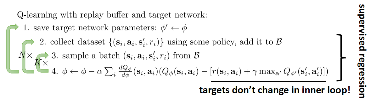
The target value every step, so the network is hard to converage, we’ll need to use another less-changed network.

If we take $K=1$ then we’ll have DQN:

1. take some action $a_i$ and observe $(s_i, a_i, s'_i, r_i)$, add it to $\mathcal{B}$, the actions were generated by $\phi$ and we might use epsilon-greedy here.
2. sample mini-batch $(s_j, a_j, s'_j, r_j)$ from $\mathcal{B}$ uniformly
3. compute $y_j = r_j + \gamma \max_{a'_j}Q_{\phi'}(s'_{j}, a'_j)$ using target network $Q_{\phi'}$
4. $\phi \leftarrow \phi - \alpha \sum_j\frac{\partial Q_\phi(s_j, a_j)}{\partial \phi}(Q_\phi(s_j, a_j) - y_j)$
5. update $\phi'$: copy $\phi$ every N steps

This way would lead the step right after the update of $\phi'$ to be only 1 step older, and the step right before to be the oldest. We could use Polyak Averaging (an optimization technique that sets final parameters to an average of recent parameters visited in the optimization trajectory) to be fair to every step.

When update $\phi'$, now we do:

$\phi' \leftarrow \tau \phi' + (1 - \tau) \phi$

For a more general view, q-learning with replay buffer and target networks is as follows:

Improve Q-learning

Problem: Overestimate the Q Value

Q-learning tends to overestimate the q value, because we calculate $y_j$ as follows:

$y_j = r_j + \gamma \underbrace{\max_{a'_j}Q_{\phi'}(s'_{j}, a'_j)}_{\text{here's the problem}}$

Because $E[\max(X_1, X_2)] \geq \max(E[X_1], E[X_2])$, and $Q \leftarrow r + \gamma E$, the q-learning will overestimate the true q value.

Solution: Double Q-learning

Note that we select action $a'$ from $Q_{\phi'}(s', a')$, and we also estimate q-value using it, so:

$\max_{a'}Q_{\phi'}(s', a') = \max_{a'}\underbrace{Q_{\phi'}}_{\text{value also from }Q_{\phi'}}(s', \underbrace{\argmax_{a'}Q_{\phi'}(s',a')}_{\text{action selected from }Q_{\phi'}})$

If $Q_{\phi'}(s', a')$ has noise, it would be multiplied. Thus we use two separate networks to choose the action and evaluate value.

$\begin{aligned} Q_{\phi_A}(s', a') &\leftarrow r + \gamma Q_{\phi_B}(s', \argmax_{a'} Q_{\phi_A}(s', a')) \\ Q_{\phi_B}(s', a') &\leftarrow r + \gamma Q_{\phi_A}(s', \argmax_{a'} Q_{\phi_B}(s', a')) \end{aligned}$

In practice, we already have target network and predict network, so we will use them as $\phi_A, \phi_B$

So a double q-learning will be:

$y = r + \gamma \max_{a'}Q_{\phi'}(s', \argmax_{a'}Q_\phi(s', a'))$

Note we use predict network $Q_\phi$ to choose actions, use target network $Q_{\phi'}$ to evaluate the value.

Overall this double-q network helps a lot in practice, and it has no downsides.

Multiple Steps

Since we calculate q-learning target by:

$y_{j,t} = r_{j,t} + \gamma \max_{a_{j, t+1}}Q_{\phi'}(s_{j,t+1}, a_{j, t+1})$

The $r_{j,t}$ is the only values that matter if $Q_{\phi'}$ is bad, and $Q_{\phi'}$ is the only values that matter if $Q_{\phi'}$ is good. So if our $Q_{\phi'}$ is bad at first, we may get stuck. If we calculate rewards at multiple steps, we could avoid this problem.

Like in actor-critic, we now have:

$y_{j,t} = \sum_{t'=t}^{t+N-1} \gamma^{t-t'}r_{j,t'} + \gamma^N \max_{a_{j, t+N}}Q_{\phi'}(s_{j,t+N}, a_{j, t+N})$

But this only works on on-policy.

In practice, just ignore this restriction and apply it to off-policy, it still works well somehow…

Countinuous Actions

To find the $\argmax_{a'}Q_{\phi'}(s', a')$ is easy when actions are discreate, but when actions are continuous, it would take much time.

Approximate

We could approximate the $\argmax_{a'}Q_{\phi'}(s', a')$ by using monte-carlo like methods:

$\max_a Q(s, a) \approx \max \{ Q(s, a_1), Q(s, a_2), \dots Q(s, a_n)\}$

$(a_1, a_2, \dots, a_N)$ are sampled from some distribution

Works well for about 40 dimensions.

Choose Easily Maximizable Q-functions

At the cost of reducing the representation capacity of q-function, we could make $\argmax_aQ$ and $\max_aQ$ very easy, for example we could use NAF/Normalized Advantage Functions

$Q_\phi(s,a) = -\frac{1}{2}(a - \mu_\phi(s))^TP_\phi(s)(a - \mu_\phi(s))+V_\phi(s)$

and we get:

$\begin{aligned} \argmax_a Q_\phi(s,a) &= \mu_\phi(s) \\ \max_aQ_\phi(s,a) &= V_\phi(s) \end{aligned}$

ddpg: learn an approximate maximizer

train a network $\mu_\theta(s)$ so that $\mu_\theta(s) \approx \argmax_{a}Q_\phi(s, a)$

ddpg:

1. take some action $a_i$ and observe $(s_i, a_i, s'_i, r_i)$, add it to $\mathcal{B}$, the actions were generated by $\phi$ and we might use epsilon-greedy here.
2. sample mini-batch $(s_j, a_j, s'_j, r_j)$ from $\mathcal{B}$ uniformly
3. compute $y_j = r_j + \gamma Q_{\phi'}(s'_{j}, \mu_{\theta'}(s'_j))$ using target network $Q_{\phi'}$ and $\mu_{\theta'}$
4. $\phi \leftarrow \phi - \alpha \sum_j\frac{\partial Q_\phi(s_j, a_j)}{\partial \phi}(Q_\phi(s_j, a_j) - y_j)$
5. $\theta \leftarrow \theta + \beta \sum_j \frac{\partial{Q_\phi}}{\partial{\theta}}$
6. update $\phi', \theta'$: eg Polyak averaging

Implement

Adam as the optimizer works better.
Remember to run using different random seeds.